For single-cell data, cell-level network analysis can be performed based on joint similarity in alpha chain sequence and beta chain sequence.
We simulate some toy data to demonstrate the usage.
set.seed(42)
library(NAIR)

dat <- simulateToyData(chains = 2)
head(dat)
#>        AlphaSeq        BetaSeq Count UMIs SampleID
#> 1 TTGAGGAAATTCG TTGAGGAAATTCGG  3095    4  Sample1
#> 2 GGAGATGAATCGG  GGAGATGAATCGG  3057    6  Sample1
#> 3 GTCGGGTAATTGG GTCGGGTAATTGGG  3575    8  Sample1
#> 4 GCCGGGTAATTCG GCCGGGTAATTCGG  3994    7  Sample1
#> 5 GAAAGAGAATTCG GAAAGAGAATTCGG  3670    3  Sample1
#> 6 AGGTGGGAATTCG  AGGTGGGAATTCG  4076    5  Sample1
The input data is assumed to have the following format:
- Each row corresponds to a unique cell
- The data contains separate columns for alpha chain sequence and beta chain sequence
Dual-chain network analysis can be performed using
buildRepSeqNetwork() (or
generateNetworkObjects()) by supplying a length-2 vector to
the seq_col parameter:
- First entry should reference the column for alpha chain sequence
- Second entry should reference the column for beta chain sequence
# Build network based on joint dual-chain similarity
network <- buildNet(dat,
                    seq_col = c("AlphaSeq", "BetaSeq"),
                    count_col = "UMIs",
                    node_stats = TRUE,
                    stats_to_include = "all",
                    cluster_stats = TRUE,
                    color_nodes_by = "SampleID",
                    size_nodes_by = "UMIs",
                    node_size_limits = c(0.5, 3)
)
We print the network graph plot with labels added for the largest two clusters:
addClusterLabels(network$plots$SampleID, network, top_n_clusters = 2, size = 8)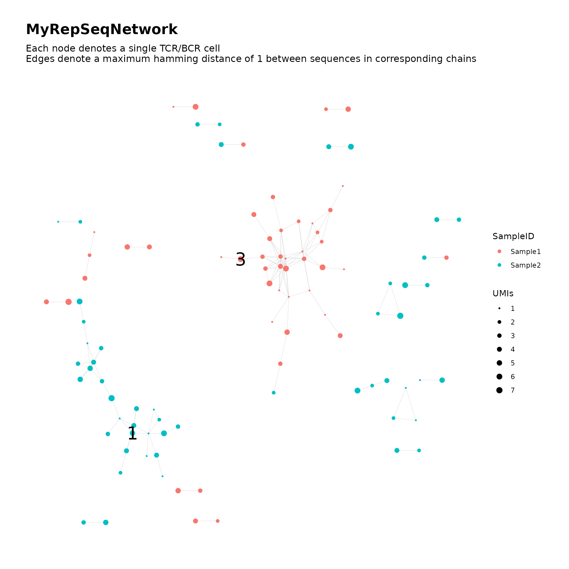
The list returned buildRepSeqNetwork() the following
items:
names(network)
#> [1] "details"          "igraph"           "adjacency_matrix" "adj_mat_a"
#> [5] "adj_mat_b"        "node_data"        "cluster_data"     "plots"
Notice that the list contains three adjacency matrices:
adjacency_matrix corresponds to the network based on joint
similarity in both chain sequences, while adj_mat_a
corresponds to the network based only on similarity in the alpha-chain
sequence (and similarly for adj_mat_b).
The cluster-level data contains sequence-based cluster statistics for each of the alpha and beta chain sequences:
head(network$cluster_data)
#>   cluster_id node_count eigen_centrality_eigenvalue eigen_centrality_index
#> 1          1         15                    3.680389           6.385488e-01
#> 2          2         13                    4.419380           6.131393e-01
#> 3          3         16                    7.257172           5.291669e-01
#> 4          4         10                    3.750958           6.107669e-01
#> 5          5          3                    1.414214           5.857864e-01
#> 6          6          3                    2.000000           8.881784e-16
#>   closeness_centrality_index degree_centrality_index edge_density
#> 1                  0.4497821               0.3190476    0.1809524
#> 2                  0.4357891               0.3141026    0.2692308
#> 3                  0.4650078               0.3250000    0.3416667
#> 4                  0.4889192               0.3555556    0.3111111
#> 5                  1.0000000               0.3333333    0.6666667
#> 6                  0.0000000               0.0000000    1.0000000
#>   global_transitivity assortativity diameter_length max_degree mean_degree
#> 1           0.2884615   -0.16503588               6          7        2.60
#> 2           0.3802817   -0.15180055               7         11        4.00
#> 3           0.6328125   -0.08424855               6         12        5.81
#> 4           0.3750000   -0.33425414               6          6        2.90
#> 5           0.0000000   -1.00000000               3          2        1.67
#> 6           1.0000000           NaN               2          2        2.00
#>   mean_A_seq_length mean_B_seq_length A_seq_w_max_degree B_seq_w_max_degree
#> 1             12.13             12.87       AAAAAAAAATTC      AAAAAAAAATTCG
#> 2             13.00             13.08      GGGGGGGAATTGG      GGGGGGGAATTGG
#> 3             13.00             13.94      GGGGGGGAATTGG     GGGGGGGAATTGGG
#> 4             12.00             12.00       AAAAAGAAATTG       AAAAAGAAATTG
#> 5             13.00             14.00      AGGGGAGAATTGG     AGGGGAGAATTGGG
#> 6             13.00             14.00      AAAAAAGAATTGC     AAAAAAGAATTGCG
#>   max_count agg_count A_seq_w_max_count B_seq_w_max_count
#> 1         6        42      AAAAAAAAATTC      AAAAAAAAATTC
#> 2         6        28     GGGGTGGAATTGG     GGGGTGGAATTGG
#> 3         6        49     GGGGAGAAATTGG    GGGGAGAAATTGGG
#> 4         7        39      AAAGAAAAATTG      AAAGAAAAATTG
#> 5         5        10     AGGGGAGAATTGG    AGGGGAGAATTGGG
#> 6         2         4     AGAAAAGAATTGC    AGAAAAGAATTGCG
The remainder of the output and customization follows the general case for
buildRepSeqNetwork().